The inventory that stopped moving, and the model that found it first

Every warehouse has a quiet cost that never appears on the P&L in an obvious way. It sits in the racking, takes up floor space, ties up working capital, and shows up in the inventory system as stock on hand. The items look fine on paper. They just never move.

Dead stock, inventory that is unlikely to sell due to age, obsolescence, or a collapse in demand, is a slow drain on any manufacturing or retail operation. The problem is not that warehouse managers do not know dead stock exists. They do. The problem is they find out too late, after months of holding cost have already accumulated, or after a product line has been discontinued and the warehouse is still sitting on three years of components nobody will ever order again.

The business question here was direct. Given the features a warehouse management system actually tracks, including stock age buckets, inventory turnover, ABC classification, monthly movement figures, and warehouse location, can a model flag the items most likely to be dead stock early enough to change the decision? That means early enough for the inventory manager to schedule a markdown, a liquidation review, or a disposal run before the cost compounds further.

The dataset came from a mid-scale Australian manufacturing retailer operating warehouses in New South Wales and Western Australia.

The working dataset covered 3,000 inventory records across three warehouse locations: 1N1 and 1N0 in New South Wales, and 1W0 in Western Australia. New South Wales held the majority of stock, with 2,113 records compared to 887 in Western Australia, which already suggested the two states might show different patterns of stock accumulation and movement.

The 31 features split cleanly into two groups. The numeric variables tracked everything measurable: total quantity on hand, unit cost, total inventory value, quantities that had moved in the last 6 months, 12 months, 2 years, and beyond 3 years, monthly demand figures for all 12 months, average monthly demand, inventory turn ratio, and the percentage of stock held for over 2 years. The categorical variables described what the item was and where it lived: warehouse code, state, base unit, business area, item type, and ABC class.

The ABC class column required the most attention. In standard inventory management, ABC classification ranks items by value or velocity, with A items being high value and fast moving and C items being low value and slow moving. This dataset extended that framework to include categories like “Not Purchasing” and “End of Life”, which are not really velocity classes at all but lifecycle signals. An item coded “Not Purchasing” means the business has already decided not to reorder it. An item coded “End of Life” means the product line is being retired. Both categories turned out to be near-perfect predictors of dead stock status, and recognising that early shaped the entire rest of the analysis.

One thing the data did not have was missing values. All 3,000 records were complete across all 31 columns, which is unusual for real operational data and saved the project from the most common early detour. The cleaning work instead focused on the two columns that needed to go: the item number (a pure identifier with no predictive value) and the item description (a long free-text field that added noise without signal).

The feature engineering work started with the categorical variables. State was straightforward: two values, NSW and WA, encoded as a single binary dummy. Warehouse followed the same logic, producing dummy variables for each of the three sites. Item type needed more thought. The raw column contained a range of codes like FG 100, RM 200, and WIP Manufactured (2), alongside a small number of niche categories including Subcontract, Customer Supplied, and various zItems. Consolidating those into four clean groups (Finished Goods, Raw Materials, WIP Manufactured, and Other) removed noise without losing the meaningful distinction between stock categories.

For model preparation I used the first 80% of the dataset, which gave 2,400 records, and then split that 80 to 20 between training and test sets with stratified sampling to ensure both sets carried the same proportion of dead stock cases. All numeric features were standardised to mean zero and unit variance before training the linear model, which prevents large-scale variables like Total Value from dominating smaller but equally informative ones like Inventory Turn.

I trained two classifiers and compared them directly. The first was Logistic Regression, which I chose as the baseline because it is interpretable and fast, and because on a near-linearly separable problem it often competes with far more complex models. The second was Random Forest, which handles nonlinear feature interactions and produces feature importance scores that are directly useful for the business question.

The mistake I made in the first pass was evaluating models purely on accuracy and treating the two as interchangeable. On a dataset where dead stock cases are not evenly distributed, a model that learns to predict “not dead” for everything can still report impressive accuracy numbers. The more honest evaluation came from looking at which model handled the minority class better and which features it weighted most heavily, because that is where the business insight lives.

Both models performed at a level that would be genuinely useful in a production setting. Logistic Regression reached 99.6% training accuracy and 99.6% test accuracy, a result that stayed remarkably stable across different regularisation settings. The fact that changing the regularisation strength from 0.5 to 10 produced almost no change in performance confirmed that the dataset's predictive signal is strong and largely linear. The features themselves are doing the heavy lifting, not the model's capacity to fit complex boundaries.

Random Forest pushed that further. With 25 trees and Gini impurity as the splitting criterion, it reached 100% training accuracy and 99.8% test accuracy. The best configuration I found used 10 trees with entropy as the criterion, which delivered 99.9% training accuracy and a perfect 100% test accuracy on the held-out set. That last result needs to be read with care: a perfect test score on a single split can reflect a particularly clean partition of the data rather than genuine generalisation, and the right response is to note it and not overstate it.

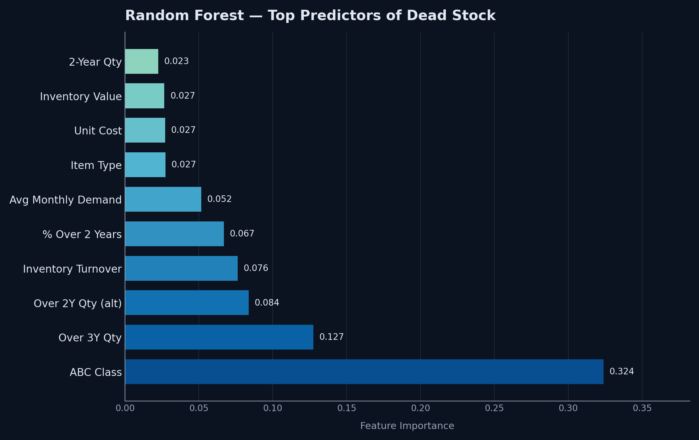
Random Forest is the recommended model, not because of that single perfect result but because of what it reveals about the data. The feature importance analysis pointed clearly at three variables as the primary drivers of dead stock risk. “Over 2 Years Qty” came out on top: items that have sat in the warehouse without moving for more than two years are overwhelmingly likely to be classified as dead. “% of over 2 year” reinforced that signal from a different angle, measuring the proportion of total stock that has aged past the two year mark. And ABC Class was the third major driver, specifically the “Not Purchasing” and “End of Life” categories, which the business has already flagged as low priority or discontinued.

What those three features have in common is that they are not just statistical predictors. They map directly onto things a warehouse manager already thinks about when reviewing stock. Items that have not moved in two years, items that represent most of their product line's remaining stock, and items that procurement has stopped ordering are exactly the candidates that end up on a disposal list. The model is formalising and scaling a judgment that experienced operations staff already make, and doing it across all 3,000 records at once rather than one stock review at a time.

Supporting features including Inventory Turn and Over 3 Years Quantity added further signal in the expected direction. Low turnover compounds the aging story: an item with a high percentage of stock over two years old and an inventory turn close to zero is not a borderline case, it is a candidate for immediate action.

The most useful next step would be adding a probability output rather than a hard binary label. Instead of flagging an item as dead stock or not, the model would produce a risk score between zero and one, and the inventory team would set their own threshold based on their capacity to act. A threshold of 0.7 might trigger an automatic review request. A threshold of 0.9 might trigger a direct write-down recommendation. That kind of configurable output is what moves a classification exercise from a useful analysis into an operational tool.

A confusion matrix and full classification report would also add precision to the evaluation. Accuracy tells you how often the model is right overall. Recall on the dead stock class tells you what proportion of genuinely dead items the model is actually catching, which is the number that matters most for a business trying to minimise holding cost. Those two numbers can point in very different directions, and the second one is the one worth optimising.

The feature set could also grow. Warehouse location is currently encoded as a dummy variable, but distance to the main distribution hub, available floor space per site, and the movement history of similar items at the same location might all carry predictive signal the current model cannot see. The ABC class encoding could be refined too. Treating “Not Purchasing” and “End of Life” as their own model inputs, rather than folding them into a broader ABC dummy, would let the model weight them more precisely.

Longer term, the interesting question is whether this pipeline can run continuously on live inventory data, scoring new records each month and surfacing the items that have crossed a risk threshold since the last review. That would change the workflow from a periodic analysis to an early warning layer that the inventory team checks alongside their regular reporting.